The Design, Construction and Flying of a Flying Wing
By Art Kresse
The design of a Flying Wing is a different aerodynamic challenge than for a conventional planform. The key issue is longitudinal (pitch) stability. Almost as important is yaw stability and control. I will deal with the pitch problem first.
The problem arises because there is no conventional horizontal stabilizer. For conventional configurations the existence of that stabilizer way behind the CG reduces the stability problem to a matter of adjusting the relative incidence of the wing and tail and the position of the CG. Whether or not the wing is stable by itself is unimportant. For a flying wing the pitch stability of the wing alone is of primary importance. Virtually all conventional wing sections, when right side up, are unstable. By the same token the same sections flying upside down are stable but not very efficient. Because of these peculiarities, a good part of the aerodynamic design involved selecting airfoil sections and the determining the required twist or washout. The other part was the planform or layout of the complete wing.
I used the computer for much of this process. The necessary calculations can be done with a hand calculator but the computer speeds up the process immensely and makes changes a piece of cake. For the design purpose I needed several major software elements. They are:
- A source of airfoil section coordinates.
- A way to analyze the sections to determine how the behave at the low speeds (Reynolds Number) that our models fly at.
- A way to estimate the performance of the complete wing.
- And finally a way to draw the wing ribs or templates that will be required.
The University of Illinois Dept of Aeronautical and Astronautical Engineering has published a large number of airfoil sections. Some these have been tested in their low speed wind tunnel (a fellow club member, Ron Bozzonetti has contributed a model wing for this project). The airfoil sections are available on the Internet1. Uiuc stands for the Uof Illinois at Urbana-Champaign and Prof. Selig is the chairman of the Applied Aerodynamics Group. The file to download is "coord960304.tar.gz". What to do next is a bit involved which I'll describe later.
The airfoil section analysis I used is based on NASA TM 80210 "A Computer Program for the Design and Analysis of Low Speed Airfoils" by Richard Eppler and Dan M. Somers , August 1980. Eppler is/was a professor of aeronautics at the University of Stuttgart in Germany and is the guru of the sailplane design folks. Somers works(ed) at NASA Langley.
The computer program developed in TM 80210 has been reworked for use on a PC by a company called "Airware" and is called "Airfoil-ii". The company is located at PO Box 295 Canton, CT 06019. As stated in the title the software works both in the design mode and the analysis mode. In the design mode you specify a desired velocity distribution over the wing (determined by guess and by golly) and the program gives you back a wing section, including the coordinates. In the analysis mode you provide section coordinates and the program gives back the aerodynamic performance (lift, drag, moments etc. just like in a wind tunnel test). There is other software available at the uiuc location on the Internet (for a price). For all I know it may be the same as Airfoil-ii. I am not about to spend more money to find out. I have tried "Airfoil-ii" and it works fine.
Ultimately, I selected the method developed in 1937 by Ray Alexander at NACA2 and adapted it for use here.
RIB PLOTTING
The rib or template plotting was done with a software, software called "Compufoil3". This is a rather well known at least to the sailplane weenies. It can be made to accept the airfoil section data that is downloaded from the U of Illinois. The same data was loaded into Design Cad which I used to do the overall design of the flying wing.
The software comes preloaded with a lot of airfoils including, I believe, some of those in the U of Illinois list. The software has provisions for modifying the airfoils and outputting coordinates. These revised coordinates can then be fed back into AIRFOIL-ii to get its characteristics. I used this feature to examine reflexed trailing edges which is a way to get stable sections for a flying wing.
The airfoil coordinate data that I used are available on the Internet at the UIUC source cited earlier under the filename "coord960304.tar.gz". The downloaded file is a list of airfoil id numbers that can be clicked on to get the coordinate listing. This listing does not give any clue as to what the airfoil looks like. Right next to the *.dat file is a *.gif file by the same name. By clicking on this filename you get a picture of the airfoil. I selected the file "e325.dat" and "e325.gif". The accompanying one line description says that this is a flying wing airfoil. This is about as good a clue that the file provides as to what the airfoil is good for. There is no aerodynamic performance data. Both of these files can be saved to disk and/or printed out. I saved them to a floppy for further use. To see what the files look like after they have been saved and you a no longer in your Internet browser a viewer is needed. For the data file the viewer (and editor) must be ASCII editor, the DOS "Editor" works fine or the Windows "notepad" editor is OK also. For the gif file, "VuePrint-Pro" which is a useful shareware graphics viewer, is suggested. The data shown in this column was imported using the standard WordPerfect "graphics " menu. Because WP does not accept *.gif files I had to re-save the file as a *.pcx file . This manipulation can easily be done in VuePrint-Pro. The airfoil coordinates are shown below. In order to use the coordinates to plot the airfoil in DesignCad some more manipulation is required. In the "Files" menu of DesignCad, select "File Convert". The input filename is (in this case) eppl325.txt. The input file type is "xy" and the output file type is dw2. Be sure to edit eppl325.txt to remove the header which names the airfoil type. DesignCad does not recognize the text and will return an error if it is left in. If you neglect to specify where you want the converted file to go you will have to look for it. Usually it goes in the directory that DesignCad is in. You can now load the file into a DesignCad window in the usual way. For some unfathomable reason when you do this into an empty window the airfoil shows up as a small spot one unit wide in a screen that is several hundred units wide. Set a point on the spot and "zoom" with a factor of about 100 and the airfoil shows up as a reasonable size. At this point you have an airfoil that can be manipulated for airplane design purposes. For airfoil performance we need to get the coordinate data into "AIRFOIL-ii".
The interesting feature of the particular airfoil that I chose is the slightly reflexed trailing edge. This has considerable effect on the stability of the airfoil. It is found on most sections that are used for flying wings.
In order to calculate the airfoil properties the airfoil coordinates for all of the sections of the wing are required. "CompuFoil" performs this task. It also has the very useful capability to "loft" the intermediate ribs when provided the root and tip rib coordinates and put all the spars and sheeting cutouts in the right place. As you might imagine this is an enormous time saver for tapered wings. I chose old faithful Clark-Y for the root section and the Eppler 325 as the tip section to illustrate the process. It would be hard to find two more different sections to try to loft together. It turned out that this combination leads to workable design.
For preliminary design I selected a wing with an 80" span, an aspect ratio of eight, an area of 800 square inches, a taper ratio of 1/2 and a sweep of 20 . This gives a root chord of 13.333", a tip chord of 6.666" and a mean chord of 10". This also turned out to be a workable configuration and became permanent.
|
The "Airfoil-ii" program requires the input airfoil coordinates in a very specific format. It must be ASCII without tabs and in two arrays of ten columns each as shown in earlier. In addition the array must start with the coordinates of the trailing edge, work forward over the top of the airfoil to the leading edge then over the bottom, and back to the trailing edge. In the text I split the array into two parts for space reasons. For input to "airfoil-ii" the file must not be split in this manner.) The number of coordinate points must be divisible by 4. The trailing edge is listed twice, at the start and at the end. A typical listing will have 69 (68+1) lines. "CompuFoil" puts a number of extraneous elements in the file which have to be removed e.g."eof" characters, tabs and labels. If this is not done properly "Airfoil-ii" will reject it.
Airfoil-ii is a FORTRAN program that originally required the old IBM card for inputs. The author did a minimal amount of work to adapt the code to an interactive PC program that that runs in DOS. Because of this the input routine is tedious and not intuitive but once set up it is acceptable. The output of the program is two forms. The visual output is a graphics plot on screen. This can be plotted immediately if you live in the old Windows 3.1 or DOS world. I found to my chagrin that graphics driver in Windows 95 will not accept the output for printing. I have not been able to find the author of the program to see if he has written an
|

The top curve is for Rib 0 (root rib) and the others are in sequence. The curve for the tip rib (rib 40) displays some strange characteristics. Most interesting are the breaks in the curve at both high and low angles of attack the other is the break in the slope at about 6 angle of attack. I do not know whether to attribute these anomalies to the reflexed trailing edge or to the strong possibility that the calculations fail at the low Reynolds Number at the tip (Re=250000). It may in fact be a combination of these problems. Sections with reflexed trailing edges are known to have poor performance (as do ordinary airfoils such and the Clark-Y when upside down). their chief advantage is the positive moment about the aerodynamic center which makes the solution to the stability problem a bit simpler for flying wings.
The data for Rib 0 (Clark-Y) is very close to the experimental data for the root Reynolds Number (Re=500000). This gives me some confidence in the results for the other sections. The lofted section (Rib 24) falls where it should, midway between the root and tip and is well behaved. If you examine the profiles closely you can see the start of the development of the reflex. The key is the curve of the lower surface of rib 24. The lower surface for the Clark-Y is essentially flat from the 20% point to the trailing edge.
For the complete wing calculations the only data of importance from these curves is the 0-intercept point and the slope of the straight portions of the curve. The nonlinear portions of the curve are much more difficult to deal with analytically for the complete wing (in other words too damn hard) and not really needed for determining the pitch stability of models.
|

The other section performance parameters are the Drag and Pitching moment Coefficients. These are shown for all three sections in figures 3 and 4. In figure 3 the drag is plotted vs angle of attack. In the working range of angle of attack (-2 to +5 deg) the drag for the three sections is virtually identical (except for the anomalous behavior of rib 40 at the extremes). It is also almost constant in that region at about 0.01. This is in accord with first order theory.
|

The moment coefficients about the 25% chord point presented in figure 4 are roughly constant for small angles of attack. If they were calculated about the aerodynamic center they would be constant. (Note: the ribs start with 0 at the top and work down). Again except for the extremities the curves behave as expected. For the complete wing the numbers that I need are the constant moment about the aerodynamic center. To get these I plotted the moment versus lift and took the value of moment at cl=0 for each of the ribs separately.
Some comments on the software are in order. The "compuFoil" software is excellent and provides much more capability than I have used so far. In particular it draws all the ribs including cutouts for sheeting, spars, leading edges and jig alignment holes with washout if desired. It contains a very large library of wing sections and a profile generator for NACA sections. It is available from the author: A demonstration program is available at his web site "http://ourworld.compuserve.com /homepages/compufoil/".
The "airfoil-ii" program has limitations at low Re. It calculates the boundary layer thickness using the velocity and pressure distributions based on no boundary layer (1st approx). The boundary layer effects the pressure and velocity and strictly speaking the calculations of the velocity and pressure should be repeated with the shape changed by the "displacement thickness". For a precise solution this is repeated until no more change is noted. Such a program is available from Proof Drela at MIT. The license for the program to non commercial users is $5000!!!
Another program called "Panda" is available from Desktop Aeronautics Inc. It has a web page and searching for the name will get you there. I have talked to them and used their demonstration program which is available on the Internet. In terms of accuracy it seems to be no better than "airfoil-ii". It uses the same first approximation for the boundary layer. It is easier to use in the sense that it is interactive. You can change the shape of the section on the screen with the mouse and watch the pressure and velocity distribution plots change with little delay. If I had not already spent a bunch of money for "airfoil-ii" I probably would go for "Panda" but as it is I got all I needed from "airfoil-ii". A big problem is that there is no technical support or updates that you would ordinarily expect.
The wing data presented above applies only to wing sections. Another way to look at it is that they apply to wings of infinite aspect ratio. I don't know how to build such a wing so we have to find a way to adjust the data to account for the fact that a real wing is finite. Like everything else in this world this will be an approximate solution.
The earliest reference that I have that treats this problem is a book by H. Glauert4 published in 1926 and republished periodically ever since. There have been numerous extensions of Glauert's work. The one that is classic and is the basis for what appears in most early texts is the previously cited work by Ray Anderson at NACA . Anderson's paper is suitable for almost anything that we design in the model world. I say almost because it falls apart completely for things like the flying lawnmower and other very low aspect ratio flying machines. It also has problems for swept wings because of the "cross flow" or flow along the wing which increases with sweep angle. Nevertheless for sweep angles of up to around 20 it gives reasonable results.
|

I struggled for bit for a way to present the calculations in some intelligible and brief way and gave up. The method involves lengthy spreadsheet arrays using numbers that are extracted from Anderson's paper. This would take more time and space than can be justified. Briefly the method adds up the characteristics of each section (as determined by airfoil-ii). The angle of attack of each section is modified by the local circulation (also known as downwash) to account for the presence of the rest of the wing. "Lifting line theory" provides the basis for estimating the downwash. Note: the downwash is a result of the vortex flow around the wing which can be made visible by smoke or condensation that many of you may have observed in full scale aircraft. It is interesting to note that none of this would happen and airplanes would never fly if it were not for the boundary layer which generates the skin friction drag. (Look up D'Alembert's Paradox as an exercise for the reader.)
The result of these calculations is the lift and moment coefficient curves for the complete, finite wing with the dimensions I used last month to generate the airfoil sections. A sketch of the planform is shown in Fig 5. The aerodynamic data are shown in figures 6 and 7. Note that the curves do not extend into the nonlinear or stall region.
|


It may not be apparent but the whole reason for this exercise is to make sure that the final wing is stable in straight and level flight. By that I mean that when put into a level flight attitude it will continue that way for some time without immediately falling off into a spiral dive or some other wild gyration. From the moment curve in fig 6, I already know that the configuration is stable in pitch because the slope of the curve is negative (it slopes up to the left). This means that if the wing is disturbed in pitch the moment increases in the proper direction to return the wing to the starting angle. What is missing is proper location of the CG so that the moments are zero and the lift is supporting the weight. To determine this I needed to know the weight (gravity). I also needed to know the cruise speed of the wing (or alternatively a "design lift coefficient"). Strictly speaking if I were doing this "by the book" I would determine this using the thrust available from the engine compared to the thrust required by the drag. Enough is enough, a good ol' SWAG will get around these problems every time. To begin with I picked a light wing loading of 18 oz per square foot. Using the dimensions on fig 1 this works out to a gross weight of 6.25 pounds. Reasonable lift coefficients for straight and level flight range around 0.1 to 0.3. The formula for lift is: L=CLAV2/384 for lift in pounds, V in mph and A in square feet. For the two values of CL the equation gives V=38 and 65 mph respectively. These are a bit high but not unreasonable. The only way to change them is to decrease the wing loading or increase the wing trim CL. For the moment at least I will go with these. The moment coefficients CM corresponding to the above lift coefficients are -.08 and -.2 respectively. The formula for moment is M=(CMAV2/384)(mac) where mac is the mean aerodynamic chord, in this case 10.37". (For some reason this dimension got lost in the translation from DesignCad to WordPerfect and is missing on the figure.) Plugging in the moment coefficients and the corresponding speeds gives -3.59 and -4.18 pound-feet for the low and high speeds respectively. The negative sign indicates that these are nose down moments and they are about the 1/4 chord point of the root chord (by definitions that I used in the original equations that I didn't show). This nose down moment must be counteracted by a nose up moment of the weight of the wing acting at the CG. At this point I had not decided where the CG would be but I have complete ? control of its location when I do the detail design. The procedure is to pick the desired CG so that the airplane trims out the desired speed and then try to build it so it falls at that point. If it doesn't work out that is what those little lead weights are for. The equation for the CG location is 12(M/Weight)=xCG, where M is in pound-feet, Weight is in pounds and xCG is in inches. The negative sign indicates that the CG should be aft of the 1/4 chord point. Again plugging the numbers gives 6.73" and 8.05" for the low and high speeds respectively. These are the locations shown on the planform in fig 1.
The change in the pitching moment between low and high speed was a little bit disconcerting. Most high performance aerobatic airplanes (model or full scale) exhibit little or no trim change with speed (desirable). Sport planes both model and full scale are generally designed to pitch up when the speed increases. In this case I had a design that tucks under as speed increases (think about it!). This was not good! The only easy way I could come up with to reduce this tendency was to change the twist or washout (increase it?). I had to do a little reprogramming to investigate this problem.
The problem is easily cured of course by a bit of up-elevator (elevon) trim. This solution is equivalent to increasing the twist of the wing (more washout). That is nice but--how much? The spreadsheet developed for the initial calculations had twist included as a fixed number. What was needed was the same spreadsheet with twist as a variable parameter. Making this change was not a big deal. It took about an hour do it and verify the results. The results are summarized in Figure 8, which plots the trim CG position as a function of airspeed for a range of twist angles. The original layout had a twist of -5 (the triangle symbol). The desired curve should be at or above the horizontal line (the curve labeled with the diamond or -
|

The remaining aerodynamic design problems are the stability in roll and yaw. I will take care of the roll problem by arbitrarily using a few degrees of dihedral. The yaw stability is not so easily brushed aside. In a conventional layout the yaw stability is provided by the fin at the end of a long fuselage. The size of the fin (including the rudder part) is not too critical since the fuselage behind the CG itself acts as a fin. For the flying wing it would be nice if I could avoid putting an "ugly" stick and fin behind the wing but that is what usually is done. Another possibility is turned up winglets at the tip of the wing. After diligently reviewing all of the aero texts that are on my bookshelf I find only two that are remotely useful. One of these has been referred to before5 and it in turn refers to a much earlier work by Grant6. (Grant's book is a classic and is in the "must read" class for anyone interested in the technical history of modeling.) Because the "Center of Lateral Area" (CLA) principle of lateral stability referred to in the references requires that both the CG and the CLA be determined and these in turn require a layout of the airplane in some detail I am going to do the detailed layout first and manipulate it to get the CG and CLA "right".
Electric power was new to me so I looked to the Internet for some help. I found a useful bit of software called "MotoCalc7". This is shareware and the price was $35US. It is a simulation that calculates the performance of electric systems (motors, gearboxes, controls and props). It has a large database of motors and other components that can be selected to for a system. It is well worth the price for designers. I
|

I ran the MotoCalc program using an Astro Cobalt 05 7T #605 (there are many others in the database provided). The program allows a range of number of cells and prop diameters and pitches and gear ratios. The outputs are Amps, Watts-in, Watts-out, Efficiency, RPM, Thrust, MPH and running time. I used a gear ratio of 4:1, prop diam range of from 11" to 15", pitch range of 7" to 10" and number of cells from 8 to 15. The program outputted 138 possibilities for each cell size. For this parameter I used 1.7 AH and 5 AH.
The combination that came closest to the 447 watts output that I assumed for the glow engine 13 cells with a 14x10 prop running and 6057 RPM. It ran with an efficiency of 80.6% and consumed 42 amps! Unfortunately it only ran for 2.5 minutes. Using 5AH cells the results were almost the same but the running time increased to 7.5 minutes. The weight of the cells is a serious problem. Nicad cells weigh roughly 1.5 oz/AH. This results in a weight for the 1.7AH cell system of 2.1 lbs. and for the 5AH system of 6.1 lbs not including the weight of the motor and controls!
These weights were too high for this first go around. I completed the design using the .46 glow engine. I may reconsider and redesign it in the future for electric but some of the flight parameters will have to change if it is to get off the ground.
One of the interesting but sometimes frustrating aspects of design especially when doing it by one's lonesome is that frequently occurs that some additional data is required that requires a diversion. This has happened once before and now it is about to happen again. Before I could do a detailed layout I needed to know what is to be "laid out". I already had most of the airframe stuff but what about the insides? The driving item was the power plant. If a design "team" had done this job there would have been a Power Plants guy who would have all the necessary data lined up for the detailer to add to the layout. As it is I had not even selected the type of power plant I want to use much less do I have all of the dimensional and weight data.
Both conventional glow engines and electric motors were candidates for this application. The big question was "what Size"? To answer this question for the glow engine without resorting to a lot of detailed calculations I used a figure I have had in my files for some years. The plot is shown in Figure 9. Running the numbers for my wing and a .30 and a .46 cu in engine I got a wing cubic loading of 7.6 oz/cu ft. and engine displacement loadings of 13.6 and 20.8 lbs/cu in for the .46 and .30 cu in engines respectively. If these points were plotted on figure 2 they would lie in the "scale"-"trainer" region. I suspected that the .30 engine would be marginal for takeoff on our grass strip so for glow power I selected a .46. Besides I already had one of those and I could weigh all of the pieces for that setup.
DETAILED DESIGN
|

While I was completing the drawing I also did a weight and balance. With a full 8 oz. fuel tank the revised estimated weight was 5.55 pounds. This was well below the 6 to 6.5 lbs that I pulled out of my ear for the initial aerodynamic design. The CG came out at 6.49" aft of the mid rib 1/4 chord reference point. The desired value is 6.23". Two oz. of lead in the nose will fix that small discrepancy. I also moved the position of the Center of Lateral Area (CLA) rearward by adding to the fin area. The distance of the CLA aft of the CG is now about 1.25 inches. This is not much but it will have to do for the time being.
Those of you who read "Air and Space" from the Smithsonian may have read the article on the Northrop Flying Wing program of the late '40s. I found the article terrifying!
One of the nice things about flying wings is that once you finish the wing the airplane is almost complete. The construction is relatively straightforward and since the emphasis of this discussion is design I do not cover the details. I will be happy to respond to questions via email.
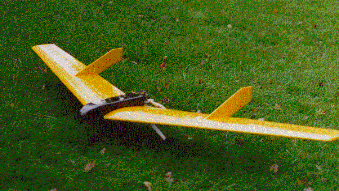
Figure 11 shows the completed with the covering and all the insides completed.
I covered the Wing with Sig "Supercoat" mostly because I had some left over from a long forgotten project. I find the "Supercoat" easier to apply than "Monocoat" mostly because it shrinks more and at a lower temperature. The slightly lower weight is insignificant. I prefer the "fabric and dope" covering but I went with the film type for weight reasons. This is in spite of the fact that I find thefabric and dope easier to apply albeit more time consuming.
I expected the visibility of the model in flight will be a problem. Except for the top and bottom , the "presented area" is small and at any distance the model will be difficult to see. To help this a bit I covered the bottom with midnight blue and the top with cub yellow. The fins help some in the side view but they are ugly and if I can get away with it some day I will remove them. The are held in only by some tabs of covering material
Finished, Ready to Fly |
As it turns out the weight is a non-issue. The final all up empty weight is 4 lbs 9 oz less muffler. This is well below my initial "guess" of 6.5 lbs and a later revision of 5.55. On top of this the center of gravity fell well within the limits calculated for stability WITHOUT BALLAST.
After a few false starts I figured out how to program my Futaba transmitter for "elevons". It works as advertised. However as the initial flight tests showed that more sophisticated programming was required.
The first successful flight of the Flying Wing took place on Feb 27, 1998. Witnesses present were Bob Yount, Pat Freeman, Dave Studenick and several other club members. Bob Yount assisted in the test. The events, attempts and adjustments leading up to this successful flight are described below.
Flight test #1
Preflight checkout OK, Controls set at maximum deflection in both directions. The control deflection at the inboard end of the elevon was about 3/4".
Taxi test OK, controlled well on ground. Accelerated smoothly and tracked OK to liftoff. Liftoff normal, climb normal to about 20 to 30-ft altitude. At this point angle of attack increased leading to an apparent stall. Aircraft tumbled over nose up several times and into the ground. No recovery possible. Damage minimal. Nose cone repaired.
Analysis: behavior symptomatic of flying wings in stall region caused by over control and lack of pitch stability in stall . Solution: decrease control deflection to preclude inadvertent stall. Add upthrust to engine (pusher) to hold nose down. Add nose weight to increase pitch stability.
Flight test #2
Behaved as before on ground. Take off as before, no pitch up or pitch instability noted but aircraft rolled right which could not be stopped with left aileron. Crash caused minor damage–broken prop and bent landing gear.
Analysis: Insufficient roll control due to reduced aileron mode deflection. Solution: Increase aileron mode deflection without increasing elevator mode deflection. This required some cogitation since the two controls are coupled. The desired effect was obtained by putting the elevator on "low rate" and aileron on "high rate." In retrospect this seems rather obvious but at the time it was not clear how the rate switches work in the elevon mode. The manual did not provide a clue. I also added exponential to the aileron control to preclude over control (I hope).
In addition I added a differential to the "aileron" mode to minimize or eliminate any adverse yaw. This is a known problem with high aspect ratio wings. Although 10 is not a particularly high aspect ratio, I did notice what seemed to be pronounced adverse yaw on the second flight. The flight was very short so I am not sure it happened. I used about 3 to 1 differential using the "ATV" mode in the transmitter. I had no idea what is the "correct" differential to use so this was an experiment.
Flight test # 3
The weather this morning was partially cloudy, temperature in the high forties with wind from the south (cross wind, what else) at from 0 to 5 knots, a beautiful day for flying. I had set up the controls before leaving home so there was little to do but fuel up and fly.
The first attempt was little more than scurrying about the runway, but it would not lift off even with full up elevator. Sitting on the ground the aircraft was slightly nose down! With the pitch control surfaces so close to the cg fore and aft they did not generate enough moment to raise the nose wheel off the ground. Bob Yount noticed that the nose wheel was bent rearward somewhat (not corrected from the previous test attempt). This leads to the nose down attitude and also a tendency of the nose wheel to "dig in" to the rough turf. This was easily corrected with some gentle metal bending.
The next attempt was successful! The aircraft tracked down the runway with no noticeable effect of the crosswind. A touch of up elevator and it was airborne. Almost no trim changes were required to get a straight and level flight at about half throttle. The aircraft is very sensitive to pitch control as expected. About three notches of up trim caused nearly vertical flight attitude.
For this first flight I stuck to straight and level flight and gentle turns. As far as I could tell the aircraft went where it was pointed which is the desired situation. Only very small control movements were required to achieve this situation. At no time did I let it get near stall attitude. This is the bad condition for flying wings since they tend to tumble when stalled. I have already demonstrated this on the first test flight.
After about five minutes of this I landed the aircraft using a rather flat long approach. Even with this, the low sink rate at idle throttle resulted in a high approach. Rather than try a go-around, I killed the engine and landed safely albeit a bit long.
Under the conditions and constraints of this flight test the aircraft exhibits good flight characteristics with no vices except for the minor requirement that the takeoff attitude be parallel to the ground or slightly nose high. It remains to be seen what happens in some of the more violent maneuvers that we subject models to. There was no noticeable adverse yaw so the differential settings must have been at least approximately correct.
The control settings that produced these results are:
Channel 1 Aileron mode
ATV=100%
EXP=-52%
D/R=85%
ATV(up surface)=100%, (dn surface)=30%
Channel 2 Elevator mode
ATV=110%
EXP=0%
D/R=40%
ATV (up)=100%, (dn)=30%
For this test I set the aileron on full rate and the elevator on low rate.
Rationale
In the case of a conventional planform the various control surfaces are all about the same distance from the axes through the cg about which they provide control (ailerons from the roll axis, elevator from the pitch axis etc.). Thus the surfaces provide roughly the same response about each axis. In the case of the flying wing the same surfaces control both roll and pitch. However, the distance to the pitch axis is much less than the distance to the roll axis. Aerodynamic control surfaces are velocity control devices, that is, they cause the control surface (and whatever it is attached to) to move with a linear velocity that is proportional to the deflection. Angular velocity (which is what we notice from the ground) is linear velocity divided by distance of the control surface to the axis of rotation. Therefor the short distance of the pitch control to its axis leads to very sensitive pitch control in comparison to the same deflection for roll control. I hope this makes sense.
Some Observations
The programmable transmitter really demonstrated its value with these control problems. Providing elevon control with different throw for the elevator and aileron modes along with exponential and differential ailerons would be a nightmare to do mechanically. The Futaba manual does not describe these combinations and is rather dense in any case but an hour or two experimentation got me what I needed.
I was very fortunate on the first two flights that they were not catastrophic. I'm not sure that if they resulted in total loss of the aircraft that I would be enthusiastic enough to start from scratch.
It might be observed that I should have been smart enough to work through the rationale before the first flight and avoided all the problems. Unfortunately I'm not that smart. (We grow too soon old and too late smart.) At least I learn from my mistakes.
Subsequent Activities
The design of "Mod 1" described above was followed by "Mod 2" which has the following specifications:
|
Span |
93" |
|
Root Chord |
20" |
|
Tip Chord |
10" |
|
Sweep |
20 deg (25% chord line) |
|
Root Section |
15% Clark Y |
|
Tip Section |
15% Eppler 325 |
|
Twist |
10 deg total aerodynamic |
|
Dihedral |
2 deg |
|
Weight |
8 lbs |
|
Power |
2-OS35s, 2 cyc, push-pull |
The layout of this design is much the same as for Mod 1 but the aspect ratio is 6 rather than 8 for Mod 1.
Using the control lessons learned from Mod 1 resulted in a completely successful first flight. The only "disconcerting" feature of both designs is their very low sink rate at idle power which makes them difficult to land in a zero wind condition. Spoilers will be used in any future design